Linear and nonlinear abstract elliptic equations with VMO coefficients and applications

Abstract

In this paper, maximal regularity properties for linear and nonlinear elliptic differential-operator equations with VMO (vanishing mean oscillation) coefficients are studied. For linear case, the uniform separability properties for parameter dependent boundary value problems is obtained in $L^p$ spaces. Then the existence and uniqueness of a strong solution of the boundary value problem for a nonlinear equation is established. In application, the maximal regularity properties of the anisotropic elliptic equation and the system of equations with VMO coefficients are derived.

MSC: 58I10, 58I20, 35Bxx, 35Dxx, 47Hxx, 47Dxx.

1 Introduction

The goal of the present paper is to study the nonlocal boundary value problems (BVPs) for parameter dependent linear differential-operator equations (DOEs) with discontinuous top-order coefficients,

$$sa(x)u^{(2)}(x)+A(x)u(x)+s^{\frac{1}{2}}{A}_1(x)u^{(1)}(x)+A_0(x)u(x)+\lambda u(x)=f(x),$$

(1)

and the nonlinear equation

$$a(x)u^{(2)}(x)+B(x,u,u^{(1)})u(x)=F(x,u,u^{(1)}),$$

where a is a complex valued function, s is a positive, λ is a complex parameter, and $A=A(x)$, $A_i=A_i(x)$ are linear and B is a nonlinear operator in a Banach space E. Here, the principal coefficients a and A may be discontinuous. More precisely, we assume that a and $A(\cdot )A^{-1}(x_0)$ belong to the operator-valued Sarason class VMO. The Sarason class VMO was first defined in [1]. In the recent years, there has been considerable interest in elliptic and parabolic equations with VMO coefficients. This is mainly due to the fact that the VMO class contains as a subspace $C(\overline{\mathrm{\Omega }})$ that ensures the extension of $L_p$-theory of operators with continuous coefficients to discontinuous coefficients (see, e.g., [2–7]). On the other hand, the Sobolev spaces $W^{1,n}(\mathrm{\Omega })$ and $W^{\sigma ,\frac{\sigma }{n}}(\mathrm{\Omega })$, $0<\sigma <1$, are also contained in VMO. Global regularity of the Dirichlet problem for elliptic equations with VMO coefficients has been studied in [2–4]. We refer to the survey [4], where an excellent presentation and relations with another similar results can be found concerning the regularizing properties of these operators in the framework of Sobolev spaces.

It is known that many classes of PDEs (partial differential equations), pseudo DEs and integro DEs can be expressed in the form of DOEs. Many researchers (see, e.g., [8–24]) investigated similar spaces of functions and classes of PDEs under a single DOE. Moreover, the maximal regularity properties of DOEs with continuous coefficients were studied, e.g., in [10, 19, 20].

Here, the equation with top-order VMO-operator coefficients is considered in abstract spaces. We shall prove the uniform separability of the problem (1), i.e., we show that, for each $f\in L^p(0,1;E)$, there exists a unique strong solution u of the problem (1) and a positive constant C depending only on p, γ, E and A such that

$$\sum _{i=0}^2{s}^{\frac{i}{2}}|\lambda {|}^{1-\frac{i}{2}}{\parallel u^{(i)}\parallel }_{L^p(0,1;E)}+{\parallel Au\parallel }_{L^p(0,1;E)}\le C{\parallel f\parallel }_{L^p(0,1;E)}.$$

Note that the principal part of a corresponding differential operator is nonselfadjoint. Nevertheless, the sharp uniform coercive estimate for the resolvent and Fredholmness are established. Then the existence and uniqueness of the above nonlinear problem is derived. In application, we study maximal regularity properties of anisotropic elliptic equations in mixed $L^{\mathbf{p}}$ spaces and the systems (finite or infinite) of differential equations with VMO coefficients in the scalar $L^p$ space.

Since (1) involves unbounded operators, it is not easy to get representation for the Green function and estimate of solutions. Therefore, we use the modern harmonic analysis elements, e.g., the Hilbert operators and the commutator estimates in E-valued $L^p$ spaces, embedding theorems of Sobolev-Lions spaces and some semigroups estimates to overcome these difficulties. Moreover, we also use our previous results on equations with continuous leading coefficients and the perturbation theory of linear operators to obtain our main assertions.

2 Notations and background

Throughout the paper, we set E to be a Banach space and $\mathrm{\Omega }\subset R^n$. $L^p(\mathrm{\Omega };E)$ denotes the space of all strongly measurable E-valued functions that are defined on Ω with the norm

$${\parallel f\parallel }_p={\parallel f\parallel }_{L^p(\mathrm{\Omega };E)}={\left({\int }_{\mathrm{\Omega }}{\parallel f(x)\parallel }_E^{p}dx\right)}^{\frac{1}{p}},1\le p<\mathrm{\infty }.$$

$\mathit{BMO}(E)$ (bounded mean oscillation) (see [21, 25]) is the space of all E-valued local integrable functions with the norm

$$\underset{B}{sup}{\int }_B{\parallel f(x)-f_B\parallel }_{E}dx={\parallel f\parallel }_{\ast ,E}<\mathrm{\infty },$$

where B ranges in the class of the balls in $R^n$ and $f_B$ is the average $\frac{1}{|B|}{\int }_{B}f(x)dx$.

For $f\in \mathit{BMO}(E)$ and $r>0$, we set

$$\underset{\rho \le r}{sup}{\int }_B{\parallel f(x)-f_B\parallel }_{E}dx=\eta (r),$$

where B ranges in the class of balls with radius ρ.

We will say that a function $f\in \mathit{BMO}(E)$ is in $\mathit{VMO}(E)$ if ${lim}_{r\to +0}\eta (r)=0$. We will call the $\eta (r)$ a VMO modulus of f.

Note that, if $E=\mathbf{C}$, where C is the set of complex numbers, then $\mathit{BMO}(E)$ and $\mathit{VMO}(E)$ coincide with the John-Nirenberg class BMO and Sarason class VMO, respectively.

The Banach space E is called a UMD (unconditional martingale difference)-space if the Hilbert operator

$$(Hf)(x)=\underset{\epsilon \to 0}{lim}{\int }_{|x-y|>\epsilon }\frac{f(y)}{x-y}dy$$

is bounded in $L_p(R,E)$, $p\in (1,\mathrm{\infty })$ (see, e.g., [26, 27]). UMD spaces include, e.g., $L_p$, $l_p$ spaces and Lorentz spaces $L_{pq}$, $p,q\in (1,\mathrm{\infty })$.

Let

$$S_{\phi }=\{\lambda \in \mathbf{C},|arg\lambda |\le \phi \}\cup \{0\},0\le \phi <\pi .$$

A linear operator A is said to be a φ-positive (or positive) in a Banach space E with the bound $M>0$ if $D(A)$ is dense on E and

$${\parallel {(A+\lambda I)}^{-1}\parallel }_{L(E)}\le M{(1+|\lambda |)}^{-1}$$

for $\lambda \in S_{\phi }$, $\phi \in (0,\pi ]$, I is an identity operator in E and $L(E)$ is the space of bounded linear operators in E. Sometimes instead of $A+\lambda I$, it will be written as $A+\lambda$ and denoted by $A_{\lambda }$. It is known [[22], §1.15.1] that there exist fractional powers $A^{\theta }$ of the positive operator A. Let $E(A^{\theta })$ denote the space $D(A^{\theta })$ with the graphical norm

$${\parallel u\parallel }_{E(A^{\theta })}={({\parallel u\parallel }^p+{\parallel A^{\theta }u\parallel }^p)}^{\frac{1}{p}},1\le p<\mathrm{\infty },-\mathrm{\infty }<\theta <\mathrm{\infty }.$$

Let $E_1$ and $E_2$ be two Banach spaces. A set $W\subset L(E_1,E_2)$ is called R-bounded (see [24, 26]) if there is a positive constant C such that for all $T_1,T_2,\dots ,T_m\in W$ and $u_{1,}{u}_2,\dots ,u_m\in E_1$, $m\in N$

$${\int }_0^1{\parallel \sum _{j=1}^m{r}_j(y)T_j{u}_j\parallel }_{E_2}dy\le C{\int }_0^1{\parallel \sum _{j=1}^m{r}_j(y)u_j\parallel }_{E_1}dy,$$

where $\{r_j\}$ is a sequence of independent symmetric $\{-1,1\}$-valued random variables on $[0,1]$.

Let $S(R^n;E)$ denote the Schwarz class, i.e., the space of all E-valued rapidly decreasing smooth functions on $R^n$. Let F denote the Fourier transformation. A function $\mathrm{\Psi }\in L^{\mathrm{\infty }}(R^n;B(E_1,E_2))$ is called a Fourier multiplier from $L_p(R^n;E_1)$ to $L_p(R^n;E_2)$ if the map $u\to {\mathrm{\Lambda }}_{\mathrm{\Psi }}u=F^{-1}\mathrm{\Psi }(\xi )Fu$, $u\in S(R^n;E_1)$ is well defined and extends to a bounded linear operator

$${\mathrm{\Lambda }}_{\mathrm{\Psi }}:L_p(R^n;E_1)\to L_p(R^n;E_2).$$

The set of all multipliers from $L_p(R^n;E_1)$ to $L_p(R^n;E_2)$ will be denoted by $M_p^p(E_1,E_2)$. For $E_1=E_2=E$, it will be denoted by $M_p^p(E)$.

Let

$$U_n=\{\beta =({\beta }_1,{\beta }_2,\dots ,{\beta }_n)\in N^n:{\beta }_k\in \{0,1\}\}.$$

Definition 1 A Banach space E is said to be a space satisfying the multiplier condition if, for any $\mathrm{\Psi }\in C^{(n)}(R^n;L(E))$, the R-boundedness of the set $\{{\xi }^{\beta }{D}_{\xi }^{\beta }\mathrm{\Psi }(\xi ):\xi \in R^n\mathrm{\setminus }0,\beta \in U_n\}$ implies that Ψ is a Fourier multiplier in $L_p(R^n;E)$, i.e., $\mathrm{\Psi }\in M_p^p(E)$ for any $p\in (1,\mathrm{\infty })$.

Definition 2 The φ-positive operator A is said to be an R-positive in a Banach space E if there exists $\phi \in [0,\pi )$ such that the set $L_A=\{A{(A+\lambda )}^{-1}:\lambda \in S_{\phi }\}$ is R-bounded.

A linear operator $A(x)$ is said to be positive in E uniformly in x if $D(A(x))$ is independent of x, $D(A(x))$ is dense in E and

$$\parallel {(A(x)+\lambda )}^{-1}\parallel \le M{(1+|\lambda |)}^{-1}$$

for all $\lambda \in S(\phi )$, $\phi \in [0,\pi )$.

Let ${\sigma }_{\mathrm{\infty }}(E_1,E_2)$ denote the space of all compact operators from $E_1$ to $E_2$. For $E_1=E_2=E$, it is denoted by ${\sigma }_{\mathrm{\infty }}(E)$.

Assume $E_0$ and E are two Banach spaces and $E_0$ is continuously and densely embedded into E. Let m be a natural number. $W^{m,p}(\mathrm{\Omega };E_0,E)$ (the so-called Sobolev-Lions type space) denotes a space of all functions $u\in L^p(\mathrm{\Omega };E_0)$ possessing the generalized derivatives $D_k^{m}u=\frac{{\partial }^{m}u}{\partial x_k^m}$ such that $D_k^{m}u\in L^p(\mathrm{\Omega };E)$ endowed with the norm

$${\parallel u\parallel }_{W^{m,p}(\mathrm{\Omega };E_0,E)}={\parallel u\parallel }_{L^p(\mathrm{\Omega };E_0)}+\sum _{k=1}^n{\parallel D_k^{m}u\parallel }_{L^p(\mathrm{\Omega };E)}<\mathrm{\infty }.$$

For $E_0=E$, the space $W^{m,p}(\mathrm{\Omega };E_0,E)$ will be denoted by $W^{m,p}(\mathrm{\Omega };E)$. It is clear that

$$W^{m,p}(\mathrm{\Omega };E_0,E)=W^{m,p}(\mathrm{\Omega };E)\cap L^p(\mathrm{\Omega };E_0).$$

Let s be a positive parameter. We define in $W^{m,p}(\mathrm{\Omega };E_0,E)$ the following parameter-dependent norm:

$${\parallel u\parallel }_{W_s^{m,p}(\mathrm{\Omega };E_0,E)}={\parallel u\parallel }_{L^p(\mathrm{\Omega };E_0)}+\sum _{k=1}^n{\parallel s{D}_k^{m}u\parallel }_{L^p(\mathrm{\Omega };E)}.$$

The space $B_{p,p}^s(\mathrm{\Gamma };E_0,E)$ is defined as a trace space for $W^{m,p}(\mathrm{\Omega };E_0,E)$ as in a scalar case (see, e.g., [[22], §3.6.1]).

Function $u\in W^{2,p}(0,1;E(A),E,L_k)=\{u\in W^{2,p}(0,1;E(A),E),L_{k}u=0\}$ satisfying the equation (1) a.e. on $(0,1)$ is said to be a solution of the problem (1) on $(0,1)$.

From [28] we have

Theorem A ₁ Suppose the following conditions are satisfied:

• (1) E is a Banach space satisfying the multiplier condition with respect to $p\in (1,\mathrm{\infty })$ and A is an R-positive operator in E;

• (2) $\alpha =({\alpha }_1,{\alpha }_2,\dots ,{\alpha }_n)$ are n tuples of nonnegative integer numbers such that $\varkappa =\frac{|\alpha |}{m}\le 1$ and $0<\mu \le 1-\varkappa$;

• (3) $\mathrm{\Omega }\in R^n$ is a region such that there exists a bounded linear extension operator from $W^{m,p}(\mathrm{\Omega };E(A),E)$ to $W^{m,p}(R^n;E(A),E)$.

Then the embedding

$$D^{\alpha }{W}^{m,p}(\mathrm{\Omega };E(A),E)\subset L^p(\mathrm{\Omega };E\left(A^{1-\varkappa -\mu }\right))$$

is continuous and there exists a positive constant $C_{\mu }$ such that

$$s^{\frac{|\alpha |}{m}}{\parallel D^{\alpha }u\parallel }_{L^p(\mathrm{\Omega };E(A^{1-\varkappa -\mu }))}\le C_{\mu }[h^{\mu }{\parallel u\parallel }_{W_s^{m,p}(\mathrm{\Omega };E(A),E)}+h^{-(1-\mu )}{\parallel u\parallel }_{L^p(\mathrm{\Omega };E)}]$$

for all $u\in W^{m,p}(\mathrm{\Omega };E(A),E)$ and $0<h\le h_0<\mathrm{\infty }$.

Theorem A ₂ Suppose all the conditions of Theorem  A₁ are satisfied. Assume Ω is a bounded region in $R^n$ and $A^{-1}\in {\sigma }_{\mathrm{\infty }}(E)$. Then, for $0<\mu \le 1-\varkappa$, the embedding

$$D^{\alpha }{W}^{m,p}(\mathrm{\Omega };E(A),E)\subset L^p(\mathrm{\Omega };E\left(A^{1-\varkappa -\mu }\right))$$

is compact.

In a similar way as in [[3], Theorem 2.1], we have the following result.

Lemma A ₁ Let E be a Banach space and $f\in \mathit{VMO}(E)$. The following conditions are equivalent:

• (1) $f\in \mathit{VMO}(E)$;

• (2) f is in the BMO closure of the set of uniformly continuous functions which belong to VMO;

• (3) ${lim}_{y\to 0}{\parallel f(x-y)-f(x)\parallel }_{\ast ,E}=0$.

For $f\in L^p(\mathrm{\Omega };E)$, $p\in (1,\mathrm{\infty })$, $a\in L^{\mathrm{\infty }}(R^n)$, consider the commutator operator

$$H[a,f](x)=a(x)Hf(x)-H(af)(x)=\underset{\epsilon \to 0}{lim}{\int }_{|x-y|>\epsilon ,}\frac{[a(x)-a(y)]}{x-y}f(y)dy.$$

From [[21], Theorem 1] and [[29], Corollary 2.7], we have

Theorem A ₃ Let E be a UMD space and $a\in \mathit{VMO}\cap L^{\mathrm{\infty }}(R^n)$. Then $H[a,f]$ is a bounded operator in $L^p(R;E)$, $p\in (1,\mathrm{\infty })$.

From Theorem A₃ and the property (2) of Lemma A₁ we obtain, respectively, the following.

Theorem A ₄ Assume all the conditions of Theorem  A₃ are satisfied. Also, let $a\in \mathit{VMO}\cap L^{\mathrm{\infty }}(R^n)$ and let η be the VMO modulus of a. Then, for any $\epsilon >0$, there exists a positive number $\delta =\delta (\epsilon ,\eta )$ such that

$${\parallel H[a,f]\parallel }_{L^p(0,r;E)}\le M\epsilon {\parallel f\parallel }_{L^p(0,r;E)},r\in (0,\delta ).$$

Theorem A ₅ Let E be a UMD space and $A(\cdot )$ uniformly R-positive in E. Moreover, let $A(\cdot )A^{-1}(x_0)\in L_{\mathrm{\infty }}(R;L(E))\cap \mathit{BMO}(L(E))$, $x_0\in R$. Then the commutator operator

$$\begin{array}{rcl}H[A,f](x)& =& A(x)A^{-1}(x_0)Hf(x)-H(A(x)A^{-1}(x_0)f)(x)\\ =& \underset{\epsilon \to 0}{lim}{\int }_{|x-y|>\epsilon ,}\frac{[A(x)A^{-1}(x_0)-A(y)A^{-1}(x_0)]}{x-y}f(y)dy\end{array}$$

is bounded in $L^p(R;E)$, $p\in (1,\mathrm{\infty })$.

Theorem A ₆ Assume all the conditions of Theorem A₅ are satisfied and η is a VMO modulus of $A(\cdot )A^{-1}(x_0)$.

Then, for any $\epsilon >0$, there exists a positive number $\delta =\delta (\epsilon ,\eta )$ such that

$${\parallel H[A,f]\parallel }_{L^p({\mathrm{\Omega }}_r;E)}\le M\epsilon {\parallel f\parallel }_{L^p({\mathrm{\Omega }}_r;E)},r\in (0,\delta ).$$

Consider the nonlocal BVP for a parameter dependent DOE with constant coefficients

(2)

where $m_k\in \{0,1\}$, a, ${\alpha }_{ki}$, ${\beta }_{ki}$ are complex numbers, s is a positive parameter, λ is a complex spectral parameter, ${\mu }_i=\frac{i}{2}+\frac{1}{2p}$, ${\theta }_k=\frac{m_k}{2}+\frac{1}{2p}$, $A_{\lambda }=A+\lambda$ and A is a linear operator in E. Let ${\omega }_1$, ${\omega }_2$ be roots of the equation $a{\omega }^2+1=0$ and let

$${\alpha }_k={\alpha }_{k{m}_k},{\beta }_k={\beta }_{k{m}_k},\mu =\left|\begin{array}{cc}{(-{\omega }_1)}^{m_1}{\alpha }_1& {\beta }_1{\omega }_1^{m_1}\\ {(-{\omega }_2)}^{m_2}{\alpha }_2& {\beta }_2{\omega }_2^{m_2}\end{array}\right|.$$

It is known that if the operator A is φ-positive in E, then operators ${\omega }_k{A}_{\lambda }^{\frac{1}{2}}$, $k=1,2$ generate analytic semigroups

$$U_{1\lambda s}(x)=e^{{\omega }_1{s}^{-\frac{1}{2}}{A}_{\lambda }^{\frac{1}{2}}x},U_{2\lambda s}(x)=e^{-{\omega }_2{s}^{-\frac{1}{2}}{A}_{\lambda }^{\frac{1}{2}}(1-x)}\mathit{\text{for}}\lambda \in S(\phi ).$$

Let

$$E_k={(E(A),E)}_{{\theta }_k,p}.$$

From [[19], Theorem 2] and [[30], Theorem 3.1], we obtain

Theorem A ₇ Assume the following conditions are satisfied:

• (1) E is a Banach space satisfying the multiplier condition with respect to $p\in (1,\mathrm{\infty })$;

• (2) A is an R-positive operator in E for $0\le \phi <\pi$ and $\mu \ne 0$;

• (3) $Re{\omega }_k\ne 0$ and $\frac{\lambda }{{\omega }_k}\in S(\phi )$ for $\lambda \in S(\phi )$, $k=1,2$.

Then

• (1) for $f\in L_p(0,1;E)$, $f_k\in E_k$, $\lambda \in S(\phi )$ and for sufficiently large $|\lambda |$, the problem (2) has a unique solution $u\in W^{2,p}(0,1;E(A),E)$. Moreover, the coercive uniform estimate holds

  $$\sum _{i=0}^2{s}^{\frac{i}{2}}|\lambda {|}^{1-\frac{i}{2}}{\parallel u^{(i)}\parallel }_{L^p(0,1;E)}+{\parallel Au\parallel }_{L^p(0,1;E)}\le C[{\parallel f\parallel }_{L^p(0,1;E)}+\sum _{k=1}^2{\parallel f_k\parallel }_{E_k}].$$

• (2) For $f_k=0$, the solution is represented as

  

  (3)

where $B_{ij}(\lambda )$ and $D_{ij}(\lambda )$ are uniformly bounded operators in E and

$$U_{0\lambda s}(x-y)=\{\begin{array}{cc}{a}^{-1}{s}^{\frac{1}{2}}{A}_{\lambda }^{-\frac{1}{2}}{U}_{1\lambda s}(x-y),\hfill & x\ge y,\hfill \\ -a^{-1}{s}^{\frac{1}{2}}{A}_{\lambda }^{-\frac{1}{2}}{U}_{2\lambda s}(x-y),\hfill & x\le y.\hfill \end{array}$$

Consider the BVP for a DOE with variable coefficients

(4)

where $a=a(x)$ is a complex valued function, s is a positive parameter, $m_k\in \{0,1\}$, ${\alpha }_{ki}$, ${\beta }_{ki}$ are complex numbers, λ is a spectral parameter, ${\theta }_k=\frac{m_k}{2}+\frac{1}{2p}$ and $A(x)$ is a linear operator in E.

Let ${\omega }_1={\omega }_1(x)$, ${\omega }_2={\omega }_2(x)$ be roots of the equation $a(x){\omega }^2+1=0$ and let

$${\alpha }_k={\alpha }_{k{m}_k},{\beta }_k={\beta }_{k{m}_k},\mu (x)=\left|\begin{array}{cc}{(-{\omega }_1)}^{m_1}{\alpha }_1& {\beta }_1{\omega }_1^{m_1}\\ {(-{\omega }_2)}^{m_2}{\alpha }_2& {\beta }_2{\omega }_2^{m_2}\end{array}\right|.$$

In the next theorem, let us consider the case that principal coefficients are continuous. The well-posedness of this problem occurs in the studying of equations with VMO coefficients. From [[19], Theorem 3] and [[21], Theorem 5.1], we get

Theorem A ₈ Suppose the following conditions are satisfied:

• (1) E is a Banach space satisfying the multiplier condition with respect to $p\in (1,\mathrm{\infty })$;

• (2) $a\in C[0,1]$, $-a\in S(\phi )$, $a(0)=a(1)$, and $\mu (x)\ne 0$ for a.e. $x\in [0,1]$;

• (3) $Re{\omega }_k(x)\ne 0$ and $\frac{\lambda }{{\omega }_k}\in S(\phi )$ for $\lambda \in S(\phi )$, $k=1,2$. a.e. $x\in [0,1]$;

• (4) $A(x)$ is a uniformly R-positive operator in E and

  $$A(\cdot )A^{-1}(x_0)\in C([0,1];L(E)),x_0\in (0,1),A(0)=A(1).$$

Then, for all $f\in L^p(0,1;E)$, $\lambda \in S(\phi )$ and for sufficiently large $|\lambda |$, there is a unique solution $u\in W^{2,p}(0,1;E(A),E)$ of the problem (4). Moreover, the following coercive uniform estimate holds:

$$\sum _{i=0}^2{s}^{\frac{i}{2}}|\lambda {|}^{1-\frac{i}{2}}{\parallel u^{(i)}\parallel }_{L^p(0,1;E)}+{\parallel Au\parallel }_{L^p(0,1;E)}\le C{\parallel f\parallel }_{L^p(0,1;E)}.$$

3 DOEs with VMO coefficients

Consider the principal part of the problem (1)

(5)

Condition 1 Assume the following conditions are satisfied:

• (1) E is a UMD space, $p\in (1,\mathrm{\infty })$;

• (2) $a\in \mathit{VMO}\cap L^{\mathrm{\infty }}(R)$, ${\eta }_1$ is a VMO modulus of a, $-a\in S(\phi )$, $\mu (x)\ne 0$;

• (3) $Re{\omega }_k(x)\ne 0$ and $\frac{\lambda }{{\omega }_k}\in S(\phi )$ for $\lambda \in S(\phi )$, $0\le \phi <\pi$, $k=1,2$. a.e. $x\in [0,1]$;

• (4) $A(x)$ is a uniformly R-positive operator in E and

  $$A(\cdot )A^{-1}(x_0)\in L_{\mathrm{\infty }}(0,1;L(E))\cap \mathit{VMO}(L(E)),x_0\in (0,1);$$

• (5) $a(0)=a(1)$, $A(0)=A(1)$ and ${\eta }_2$ is a VMO modulus of $A(\cdot )A^{-1}(x_0)$.

First, we obtain an integral representation formula for solutions.

Lemma 1 Let Condition 1 hold and $f\in L^p(0,1;E)$. Then, for all solutions u of the problem (5) belonging to $W^{2,p}(0,1;E(A),E)$, we have

(6)

where

here $B_{ij}^{\mathrm{\prime }}(\lambda )$, $D_{ij}^{\mathrm{\prime }}(\lambda )$ are uniformly bounded operators,

$$U_{\nu 0\lambda s}^{\mathrm{\prime }}(x-y)=\{\begin{array}{cc}{\omega }_1^i{a}^{-1}{s}^{(1-\nu )/2}{A}_{\lambda }^{-(1-\nu )/2}{U}_{1\lambda s}(x-y),\hfill & x\ge y,\hfill \\ -{\omega }_2^i{a}^{-1}{s}^{(1-\nu )/2}{A}_{\lambda }^{-(1-\nu )/2}{U}_{2\lambda s}(x-y),\hfill & x\le y,\hfill \end{array}$$

and the expression ${\mathrm{\Gamma }}_{2\lambda }^{\mathrm{\prime }}(x,x-y)$ is a scalar multiple of ${\mathrm{\Gamma }}_{2\lambda }(x,x-y)$.

Proof Consider the problem (5) for $a(x)=a(x_0)$ and $A(x)=A(x_0)$, i.e.,

(7)

Let $u\in C^{(2)}([0,1];E(A))$ be a solution of the problem (7). Taking into account the equality $L_{0}u=(L_0-L)u+Lu$ and Theorem A₇, we get

Setting $x=x_0$ in above, we get (6) for $u\in C^{(2)}([0,1];E(A))$. Then the density argument, using Theorem A₃, gives the conclusion for

$$u\in W^{2,p}(0,1;E(A),E),L_{k}u=0.$$

Consider the problem (5) on $(0,b)$, i.e.,

(8)

 □

Theorem 1 Suppose Condition 1 is satisfied. Then there exists a number $b\in (0,1)$ such that the uniform coercive estimate

$$\sum _{i=0}^2{s}^{\frac{i}{2}}|\lambda {|}^{1-\frac{i}{2}}{\parallel u^{(i)}\parallel }_{L^p(0,b;E)}+{\parallel Au\parallel }_{L^p(0,b;E)}\le C{\parallel (L_b+\lambda )u\parallel }_{L^p(0,b;E)}$$

(9)

holds for large enough $|\lambda |$ and $u\in W^{2,p}(0,b;E(A),E)$, $L_{bk}u=0$, $\lambda \in S(\phi )$, where C is a positive constant depending only on p, $M_0$, ${\eta }_1$, ${\eta }_2$.

Proof By Lemma 1, for any solution $u\in W^{2,p}(0,b;E(A),E)$ of the problem (8), we have

$$\begin{array}{rcl}{u}^{(i)}(x)& =& {\int }_0^b{\mathrm{\Gamma }}_{ib\lambda s}(x,x-y)\{[a(x)-a(y)]u^{(2)}(y)\\ +[A(x)-A(y)]u(y)+f(y)\}dy+f(x),\end{array}$$

(10)

where

$$\begin{array}{rcl}{\mathrm{\Gamma }}_{ib\lambda s}(x,x-y)& =& \sum _{i,j=1}^2\sum _{k=0}^{m_1}[B_{ij}^{\mathrm{\prime }}(\lambda ){\left(s^{-1}{A}_{\lambda }\right)}^{-\frac{1}{2}(2+m_k-k-i-1)}{U}_{j\lambda }(x)U_{1\lambda }(b-y)]\\ +\sum _{i,j=1}^2\sum _{k=0}^{m_2}[D_{ij}^{\mathrm{\prime }}(\lambda ){\left(s^{-1}{A}_{\lambda }\right)}^{-\frac{1}{2}(2+m_k-k-i-1)}{U}_{j\lambda }(x)U_{2\lambda }(y)]\\ +U_{\nu 0\lambda s}^{\mathrm{\prime }}(x-y),\nu =0,1,2,\end{array}$$

(11)

here $B_{ij}^{\mathrm{\prime }}(\lambda )$, $D_{ij}^{\mathrm{\prime }}(\lambda )$ are uniformly bounded operators,

$$U_{1\lambda }(x)=e^{{\omega }_1{s}^{-\frac{1}{2}}{A}_{\lambda }^{\frac{1}{2}}x},U_{2\lambda }(x)=e^{-{\omega }_2{s}^{-\frac{1}{2}}{A}_{\lambda }^{\frac{1}{2}}(b-x)}$$

and

$$U_{\nu 0\lambda s}^{\mathrm{\prime }}(x-y)=\{\begin{array}{cc}{\omega }_1^i{a}^{-1}{s}^{(1-\nu )/2}{A}_{\lambda }^{-(1-\nu )/2}{U}_{1\lambda s}(x-y),\hfill & x\ge y,\hfill \\ -{\omega }_2^i{a}^{-1}{s}^{(1-\nu )/2}{A}_{\lambda }^{-(1-\nu )/2}{U}_{2\lambda s}(x-y),\hfill & x\le y,\hfill \end{array}\nu =0,1,2.$$

Moreover, from (10) and (11), clearly, we get

$$Au(x)={\int }_0^b{\mathrm{\Gamma }}_{b\lambda s}^{\mathrm{\prime }}(x,x-y)\{[a(x)-a(y)]u^{(2)}(y)+[A(x)-A(y)]u(y)+f(y)\}dy,$$

(12)

where the expression ${\mathrm{\Gamma }}_{b\lambda }^{\mathrm{\prime }}(x,x-y)$ differs from ${\mathrm{\Gamma }}_{2b\lambda }(x,x-y)$ only by a constant.

Consider the operators

Since the operators $B_{0\lambda }$ and $B_{1\lambda }$ are regular on $L^p(0,b;E)$, by using the positivity properties of A and the analyticity of semigroups $U_{k\lambda }(x)$ in a similar way as in [[30], Theorem 3.1], we get

$${\parallel B_{i\lambda }f\parallel }_{L^p(0,b;E)}\le M|\lambda {|}^{-\frac{2-i}{2}}{\parallel f\parallel }_{L^p(0,b;E)},i=0,1.$$

(13)

Since the Hilbert operator is bounded in $L^p(R;E)$ for a UMD space E, we have

$${\parallel B_{2\lambda }f\parallel }_{L^p(0,b;E)}\le M{\parallel f\parallel }_{L^p(0,b;E)}.$$

(14)

Thus, by virtue of Theorems A₄, A₆ and in view of (10)-(12) for any $\epsilon >0$, there exists a positive number $b=b(\epsilon ,{\eta }_1,{\eta }_2)$ such that

(15)

Hence, the estimates (13)-(15) imply (9). □

Theorem 2 Assume Condition 1 holds. Let $u\in W^{2,p}(0,1;E(A),E)$ be a solution of (4). Then, for sufficiently large $|\lambda |$, $\lambda \in S(\phi )$, the following coercive uniform estimate holds:

$$\sum _{i=0}^2{s}^{\frac{i}{2}}|\lambda {|}^{1-\frac{i}{2}}{\parallel u^{(i)}\parallel }_{L^p(0,1;E)}+{\parallel Au\parallel }_{L^p(0,1;E)}\le C[{\parallel (L+\lambda )u\parallel }_{L^p(0,1;E)}+{\parallel u\parallel }_{L^p(0,1;E)}].$$

(16)

Proof This fact is shown by a covering and flattening argument, in a similar way as in Theorem A₈. Particularly, by partition of unity, the problem is localized. Choosing diameters of supports for corresponding finite functions, by using Theorem 1, Theorems A₄, A₆, A₇ and embedding Theorem A₁ (see the same technique for DOEs with continuous coefficients [19, 20]), we obtain the assertion.

Let $Q_s$ denote the operator in $L^p(0,1;E)$ generated by the problem (4) for $\lambda =0$, i.e.,

$$D(Q_s)=W^{2,p}(0,1;E(A),E,L_k),Q_{s}u=sa(x)u^{(2)}+A(x)u.$$

 □

Theorem 3 Assume Condition 1 holds. Then, for all $f\in L^p(0,1;E)$, $\lambda \in S(\phi )$ and for large enough $|\lambda |$, the problem (5) has a unique solution $u\in W^{2,p}(0,1;E(A),E)$. Moreover, the following coercive uniform estimate holds:

$$\sum _{i=0}^2{s}^{\frac{i}{2}}|\lambda {|}^{1-\frac{i}{2}}{\parallel u^{(i)}\parallel }_{L^p(0,1;E)}+{\parallel Au\parallel }_{L^p(0,1;E)}\le C{\parallel f\parallel }_{L^p(0,1;E)}.$$

(17)

Proof First, let us show that the operator $Q+\lambda$ has a left inverse. Really, it is clear that

$${\parallel u\parallel }_{L^p(0,1;E)}=\frac{1}{|\lambda |}[{\parallel (Q_s+\lambda )u\parallel }_{L^p(0,1;E)}+{\parallel Q_{s}u\parallel }_{L^p(0,1;E)}].$$

By Theorem A₁ for $u\in W^{2,p}(0,1;E(A),E)$, we have

$${\parallel Q_{s}u\parallel }_{L^p(0,1;E)}\le C{\parallel u\parallel }_{W_s^{2,p}(0,1;E(A),E)}.$$

Then, by virtue of (16) and in view of the above relations, we infer, for all $u\in W^{2,p}(0,1;E(A),E)$ and sufficiently large $|\lambda |$, that there is a small ε and $C(\epsilon )$ such that

(18)

From the estimate (18) for $u\in W^{2,p}(0,1;E(A),E)$, we get

$$\sum _{i=0}^2{s}^{\frac{i}{2}}|\lambda {|}^{1-\frac{i}{2}}{\parallel u^{(i)}\parallel }_{L^p(0,1;E)}+{\parallel Au\parallel }_{L^p(0,1;E)}\le C{\parallel (Q+\lambda )u\parallel }_{L^p(0,1;E)}.$$

(19)

The estimate (19) implies that (4) has a unique solution and the operator $Q_s+\lambda$ has a bounded inverse in its rank space. We need to show the rank space coincides with all the space $L^p(0,1;E)$. It suffices to prove that there is a solution $u\in W^{2,p}(0,1;E(A),E)$ for all $f\in L^p(0,1;E)$. This fact can be derived in a standard way, approximating the equation with a similar one with smooth coefficients [19, 20]. More precisely, by virtue of [[23], Theorem 3.4], UMD spaces satisfy the multiplier condition. Moreover, by the part (2) of Lemma A₁, given $a\in \mathit{VMO}$ with VMO modules $\eta (r)$, we can find a sequence of mollifiers functions $\{a_h\}$ converging to a in BMO as $h\to 0$ with a VMO modulus ${\eta }_h$ such that ${\eta }_h(r)\le \eta (r)$. In a similar way, it can be derived for the operator function $A(x)A^{-1}(x_0)\in \mathit{VMO}(L(E))$. □

Result 1 Theorem 3 implies that the resolvent ${(Q_s+\lambda )}^{-1}$ satisfies the following sharp uniform estimate:

$$\sum _{i=0}^2{s}^{\frac{i}{2}}|\lambda {|}^{1-\frac{i}{2}}{\parallel \frac{d^i}{d{x}^i}{(Q_s+\lambda )}^{-1}\parallel }_{L(L^p(0,1;E))}+{\parallel A{(Q_s+\lambda )}^{-1}\parallel }_{L(L^p(0,1;E))}\le C$$

(20)

for $|arg\lambda |\le \phi$, $\phi \in (0,\pi )$ and $s>0$.

The estimate (20) particularly implies that the operator Q is uniformly positive in $L^p(0,1;E)$ and generates analytic semigroups for $\phi \in (\frac{\pi }{2},\pi )$ (see, e.g., [[22], §1.14.5]).

Remark 1 Conditions $a(0)=a(1)$, $A(0)=A(1)$ arise due to nonlocality of the boundary conditions (4). If the boundary conditions are local, then the conditions mentioned above are not required any more.

Consider the problem (1), where $L_{k}u$ is the same boundary condition as in (4). Let $O_s$ denote a differential operator generated by the problem (1). We will show the separability and Fredholmness of (1).

Theorem 4 Assume

• (1) Condition 1 holds;

• (2) for any $\epsilon >0$, there is $C(\epsilon )>0$ such that for a.e. $x\in (0,1)$ and for $0<{\nu }_0<1$, $0<{\nu }_1<\frac{1}{2}$,

  

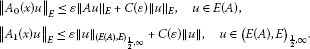
Then, for all $f\in L^p(0,1;E)$ and for large enough $|\lambda |$, $\lambda \in S(\phi )$, there is a unique solution $u\in W^{2,p}(0,1;E(A),E)$ of the problem (1) and the following coercive uniform estimate holds:

$$\sum _{i=0}^2{s}^{\frac{i}{2}}|\lambda {|}^{1-\frac{i}{2}}{\parallel u^{(i)}\parallel }_{L^p(0,1;E)}+{\parallel Au\parallel }_{L^p(0,1;E)}\le C{\parallel f\parallel }_{L^p(0,1;E)}.$$

(21)

Proof It is sufficient to show that the operator $O_s+\lambda$ has a bounded inverse ${(O_s+\lambda )}^{-1}$ from $L^p(0,1;E)$ to $W^{2,p}(0,1;E(A),E)$. Put $O_{s}u=Q_{s}u+Q_{0}u$, where

$$Q_{0}u=s^{\frac{1}{2}}{A}_1{u}^{(1)}+A_{0}u,u\in W^{2,p}(0,1;E(A),E,L_k).$$

By the second assumption and Theorem A₁, there is a small ε and $C(\epsilon )$ such that

$$\begin{array}{r}{\parallel A_{0}u\parallel }_{L^p(0,1;E)}\le C{\parallel A^{1-{\nu }_0}u\parallel }_{L^p(0,1;E)}\\ \phantom{{\parallel A_{0}u\parallel }_{L^p(0,1;E)}}\le \epsilon {\parallel u\parallel }_{W_s^{2,p}(0,1;E(A),E)}+C(\epsilon ){\parallel u\parallel }_{L^p(0,1;E)},\\ {\parallel s^{\frac{1}{2}}{A}_1{u}^{(1)}\parallel }_{L^p(0,1;E)}\le C{\parallel s^{\frac{1}{2}}{A}^{\frac{1}{2}-{\nu }_1}u\parallel }_{L^p(0,1;E)}\\ \phantom{{\parallel s^{\frac{1}{2}}{A}_1{u}^{(1)}\parallel }_{L^p(0,1;E)}}\le \epsilon {\parallel u\parallel }_{W_s^{2,p}(0,1;E(A),E)}+C(\epsilon ){\parallel u\parallel }_{L^p(0,1;E)}.\end{array}$$

(22)

In view of estimates (17) and (22), we have

$$\begin{array}{r}{\parallel A_{0}u\parallel }_{L^p(0,1;E)}<{\delta }_1{\parallel Q_{s}u\parallel }_{L^p(0,1;E)},\\ {\parallel s^{\frac{1}{2}}{A}_1{u}^{(1)}\parallel }_{L^p(0,1;E)}<{\delta }_1{\parallel Q_{s}u\parallel }_{L^p(0,1;E)}\end{array}$$

(23)

for $u\in W^{2,p}(0,1;E(A),E)$ and ${\delta }_k<1$. By Theorem 3, the operator $Q_s+\lambda$ has a bounded inverse ${(Q_s+\lambda )}^{-1}$ from $L^p(0,1;E)$ to $W^{2,p}(0,1;E(A),E)$ for sufficiently large $|\lambda |$. So, (23) implies the following uniform estimate:

$${\parallel Q_0{(Q_s+\lambda )}^{-1}\parallel }_{L(L^p(0,1;E))}<1.$$

It is clear that

Then, by above relation and by virtue of Theorem 3, we get the assertion. □

Theorem 4 implies the following result.

Result 2 Suppose all the conditions of Theorem 4 are satisfied. Then the resolvent ${(O_s+\lambda )}^{-1}$ of the operator $O_s$ satisfies the following sharp uniform estimate:

$$\sum _{i=0}^2{s}^{\frac{i}{2}}|\lambda {|}^{1-\frac{i}{2}}{\parallel \frac{d^i}{d{x}^i}{(O_s+\lambda )}^{-1}\parallel }_{L(L^p(0,1;E))}+{\parallel A{(O_s+\lambda )}^{-1}\parallel }_{L(L^p(0,1;E))}\le C$$

for $|arg\lambda |\le \phi$, $\phi \in [0,\pi )$ and $s>0$.

Consider the problem (1) for $\lambda =0$, i.e.,

(24)

Theorem 5 Assume all the conditions of Theorem  4 hold and $A^{-1}\in {\sigma }_{\mathrm{\infty }}(E)$. Then the problem (24) is Fredholm from $W^{2,p}(0,1;E(A),E)$ into $L^p(0,1;E)$.

Proof Theorem 4 implies that the operator $O_s+\lambda$ has a bounded inverse ${(O_s+\lambda )}^{-1}$ from $L^p(0,1;E)$ to $W^{2,p}(0,1;E(A),E)$ for large enough $|\lambda |$; that is, the operator $O_s+\lambda$ is Fredholm from $W^{2,p}(0,1;E(A),E)$ into $L^p(0,1;E)$. Then, by virtue of Theorem A₂ and by perturbation theory of linear operators, we obtain the assertion. □

4 Nonlinear DOEs with VMO coefficients

Let, at first, consider the linear BVP in a moving domain $(0,b(s))$,

(25)

where a is a complex valued function, and $A=A(x)$, $A_i=A_i(x)$ are possible operators in a Banach space E, where $b(s)$ is a positive continuous independent of u.

Theorem 4 implies the following result.

Result 3 Let all the conditions of Theorem 4 be satisfied. Then the problem (25), for $f\in L^p(0,b(s);E)$, $p\in (1,\mathrm{\infty })$, $\lambda \in S_{\phi }$ and for large enough $|\lambda |$, has a unique solution $u\in W^{2,p}(0,b;E(A),E)$ and the following coercive uniform estimate holds:

$$\sum _{i=0}^2|\lambda {|}^{1-\frac{i}{2}}{\parallel u^{(i)}\parallel }_{L^p(0,b;E)}+{\parallel Au\parallel }_{L^p(0,b;E)}\le {\parallel f\parallel }_{L^p(0,b;E)}.$$

Proof Really, under the substitution $\tau =xb(s)$, the moving boundary problem (25) maps to the following BVP with a parameter in a fixed domain $(0,1)$:

where

$$\tau \in (0,1),\tilde{A}=A(\tau b^{-1}(s)),{\tilde{A}}_i=A_i(\tau b^{-1}(s)).$$

Then, by virtue of Theorem 4, we obtain the assertion. □

Consider the nonlinear problem

(26)

where $m_k\in \{0,1\}$, ${\alpha }_{ki}$, ${\beta }_{ki}$ are complex numbers, $x\in (0,b)$, where b is a positive number in $(0,b_0]$.

In this section, we will prove the existence and uniqueness of a maximal regular solution of the nonlinear problem (26). Assume A is a φ-positive operator in a Banach space E. Let

Remark 2 By using [[22], §1.8], we obtain that the embedding $D^{j}Y\in E_j$ is continuous and there exists the constant $C_1$ such that for $w\in Y$, $W=\{w_{0,}{w}_1\}$, $w_j=D^{j}w(\cdot )$, $j=0,1$,

$${\parallel w\parallel }_{X_0,\mathrm{\infty }}=\prod _{j=0}^1{\parallel D^{j}w\parallel }_{C([0,b],E_j)}=\underset{x\in [0,b]}{sup}\prod _{j=0}^1{\parallel D^{j}w(x)\parallel }_{E_j}\le C_1{\parallel w\parallel }_Y.$$

Condition 2 Assume the following are satisfied:

• (1) $\eta ={(-1)}^{m_1}{\alpha }_1{\beta }_2-{(-1)}^{m_2}{\alpha }_2{\beta }_1\ne 0$ and $a(x)$ is a positive continuous function on $[0,b]$, $a(0)=a(b)$;

• (2) E is a UMD space and $p\in (1,\mathrm{\infty })$;

• (3) $F(x,{\upsilon }_0,{\upsilon }_1):[0,b]\times X_0\to E$ is a measurable function for each ${\upsilon }_i\in E_i$, $i=0,1$; $F(x,\cdot ,\cdot )$ is continuous with respect to $x\in [0,b]$ and $f(x)=F(x,0)\in X$. Moreover, for each $R>0$, there exists ${\mu }_R$ such that

  $${\parallel F(x,U)-F(x,\overline{U})\parallel }_E\le {\mu }_R{\parallel U-\overline{U}\parallel }_{X_0},$$

  where $U=\{u_0,u_1\}$ and $\overline{U}=\{{\overline{u}}_0,{\overline{u}}_1\}$ for a.a. $x\in [0,b]$, $u_i,{\overline{u}}_i\in E_i$ and

  $${\parallel U\parallel }_{X_0}\le R,{\parallel \overline{U}\parallel }_{X_0}\le R.$$

• (4) for $U=\{u_0,u_1\}\in X_0$, the operator $B(x,U)$ is R-positive in E uniformly with respect to $x\in [0,b]$; $B(x,U)B^{-1}(x^0,U)\in C([0,b];B(E))$, where the domain definition $D(B(x,U))$ does not depend on x and U; $B(x,W):(0,b)\times X_0\to B(E(A),E)$ is continuous, where $A=A(x)=B(x,W)$ for fixed $W=\{w_0,w_1\}\in X_0$;

• (5) for each $R>0$, there is a positive constant $L(R)$ such that ${\parallel [B(x,U)-B(x,\overline{U})]\upsilon \parallel }_E\le L(R){\parallel U-\overline{U}\parallel }_{X_0}{\parallel A\upsilon \parallel }_E$ for $x\in (0,b)$, $U,\overline{U}\in X_0$, ${\parallel U\parallel }_{X_0},{\parallel \overline{U}\parallel }_{X_0}\le R$ and $\upsilon \in D(A)$ and $A(0)=A(b)$.

Theorem 6 Let Condition 1 hold. Then there is $b\in (0,b_0]$ such that the problem (26) has a unique solution that belongs to the space $W_p^2(0,b;E(A),E)$.

Proof Consider the linear problem

(27)

where

$$f(x)=F(x,0),x_0\in (0,b).$$

By virtue of Result 3, the problem (27) has a unique solution for all $f\in X$ and for sufficiently large $d>0$ that satisfies the following

$${\parallel w\parallel }_Y\le C_0{\parallel f\parallel }_X,$$

where the constant C does not depend on $f\in X$ and $b\in (0,b_0]$. We want to solve the problem (26) locally by means of maximal regularity of the linear problem (27) via the contraction mapping theorem. For this purpose, let w be a solution of the linear BVP (27). Consider a ball

$$B_r=\{\upsilon \in Y,L_k\upsilon =0,k=1,2,{\parallel \upsilon -w\parallel }_Y\le r\}.$$

For $\upsilon \in B_r$, consider the linear problem

(28)

where

$$V=\{\upsilon ,{\upsilon }^{(1)}\},W=\{w,w^{(1)}\}.$$

Define a map Q on $B_r$ by $Q\upsilon =u$, where u is a solution of the problem (28). We want to show that $Q(B_r)\subset B_r$ and that Q is a contraction operator provided b is sufficiently small and r is chosen properly. For this aim, by using maximal regularity properties of the problem (28), we have

$${\parallel Q\upsilon -w\parallel }_Y={\parallel u-w\parallel }_Y\le C_0\{{\parallel F(x,V)-F(x,0)\parallel }_X+{\parallel [B(0,W)-B(x,V)]\upsilon \parallel }_X\}.$$

By assumption (5), we have

where

$$\delta (b)=\underset{x\in [0,b]}{sup}{\parallel [B(0,W)-B(x,W)]\parallel }_{B(X_0,X)}.$$

Bearing in mind

$$\begin{array}{rcl}{\parallel F(x,V)-F(x,0,)\parallel }_E& \le & \delta (b)+{\parallel F(x,V)-F(x,W)\parallel }_E+{\parallel F(x,W)-F(x,0)\parallel }_E\\ \le & \delta (b)+{\mu }_R[{\parallel \upsilon -w\parallel }_Y+{\parallel w\parallel }_Y]{\mu }_R{C}_1[{\parallel \upsilon -w\parallel }_Y+{\parallel w\parallel }_Y]\\ \le & {\mu }_R[C_{1}r+{\parallel w\parallel }_Y],\end{array}$$

where $R=C_{1}r+{\parallel w\parallel }_Y$ is a fixed number. In view of the above estimates, by a suitable choice of ${\mu }_R$, $L_R$ and for sufficiently small $b\in [0;b_0)$, we have

$${\parallel Q\upsilon -w\parallel }_Y\le r,$$

i.e.,

$$Q(B_r)\subset B_r.$$

Moreover, in a similar way, we obtain

$$\begin{array}{rcl}{\parallel Q\upsilon -Q\overline{\upsilon }\parallel }_Y& \le & C_0\{{\mu }_R{C}_1+M_a+L(R)[{\parallel \upsilon -w\parallel }_Y+C_{1}r]\\ +L(R)C_1[r+{\parallel w\parallel }_Y]{\parallel \upsilon -\overline{\upsilon }\parallel }_Y\}+\delta (b).\end{array}$$

By a suitable choice of ${\mu }_R$, $L_R$ and for sufficiently small $b\in (0,b_0)$, we obtain ${\parallel Q\upsilon -Q\overline{\upsilon }\parallel }_Y<\eta {\parallel \upsilon -\overline{\upsilon }\parallel }_Y$, $\eta <1$, i.e., Q is a contraction operator. Eventually, the contraction mapping principle implies a unique fixed point of Q in $B_r$ which is the unique strong solution $u\in Y$. □

5 Boundary value problems for anisotropic elliptic equations with VMO coefficients

The Fredholm property of BVPs for elliptic equations with parameters in smooth domains were studied, e.g., in [8, 10], also, for nonsmooth domains, these questions were investigated, e.g., in [31].

Let $\mathrm{\Omega }\subset R^n$ be an open connected set with a compact $C^{2m}$-boundary ∂ Ω. Let us consider the nonlocal boundary value problems on a cylindrical domain $G=(0,1)\times \mathrm{\Omega }$ for the following anisotropic elliptic equation with VMO top-order coefficients:

(29)

(30)

(31)

where s is a positive parameter, a, $d_i$ are complex valued functions, ${\alpha }_{ki}$ and ${\beta }_{ki}$ are complex numbers,

$$D_j=-i\frac{\partial }{\partial y_j},m_k\in \{0,1\},y=(y_1,\dots ,y_n),{\mu }_i=\frac{i}{2}+\frac{1}{2p}.$$

If $G=(0,1)\times \mathrm{\Omega }$, $\mathbf{p}=(p_1,p)$, $L^{\mathbf{p}}(G)$ will denote the space of all p-summable scalar-valued functions with a mixed norm (see, e.g., [[32], §1]), i.e., the space of all measurable functions f defined on G, for which

$${\parallel f\parallel }_{L^{\mathbf{p}}(G)}={\left({\int }_0^1{\left({\int }_{\mathrm{\Omega }}\right|f(x,y){|}^{p_1}dy)}^{\frac{p}{p_1}}dx\right)}^{\frac{1}{p}}<\mathrm{\infty }.$$

Analogously, $W^{2,2m,\mathbf{p}}(G)$ denotes the anisotropic Sobolev space with the corresponding mixed norm [[32], §10].

Theorem 7 Let the following conditions be satisfied;

• (1) $a,d_0\in \mathit{VMO}\cap L^{\mathrm{\infty }}(R)$, $a(0)=a(1)$, $-a\in S(\phi )$, $\mu (x)\ne 0$, a.e. $x\in [0,1]$;

• (2) $Re{\omega }_k\ne 0$ and $\frac{\lambda }{{\omega }_k}\in S(\phi )$ for $\lambda \in S(\phi )$, $0\le \phi <\pi$, $k=1,2$ a.e. $x\in [0,1]$;

• (3) $d_1\in L^{\mathrm{\infty }}$, $d_1(\cdot ,y)d_0^{\frac{1}{2}-\nu }(\cdot )\in L^{\mathrm{\infty }}(0,1)$ for a.e. $y\in \mathrm{\Omega }$ and $0<\nu <\frac{1}{2}$;

• (4) $a_{\alpha }\in \mathit{VMO}\cap L^{\mathrm{\infty }}(R^n)$ for each $|\alpha |=2m$ and $a_{\alpha }\in [L^{\mathrm{\infty }}+L^{{\gamma }_k}](\mathrm{\Omega })$ for each $|\alpha |=k<2m$ with $r_k\ge q$ and $2m-k>\frac{l}{r_k}$;

• (5) $b_{j\beta }\in C^{2m-m_j}(\partial \mathrm{\Omega })$ for each j, β and $m_j<2m$, , for $|\beta |=m_j$, , where $\sigma =({\sigma }_1,{\sigma }_2,\dots ,{\sigma }_n)\in R^n$ is a normal to ∂G;

• (6) for $y\in \overline{\mathrm{\Omega }}$, $\xi \in R^n$, $\nu \in S(\phi )$, $\phi \in (0,\pi )$, $|\xi |+|\nu |\ne 0$ let $\nu +{\sum }_{|\alpha |=2m}{a}_{\alpha }(y){\xi }^{\alpha }\ne 0$;

• (7) for each $y_0\in \partial \mathrm{\Omega }$, a local BVP in local coordinates corresponding to $y_0$

  

has a unique solution $\vartheta \in C_0(R_{+})$ for all $h=(h_1,h_2,\dots ,h_n)\in R^n$, and for ${\xi }^{\mid }\in R^{n-1}$ with $|{\xi }^{\mid }|+|\nu |\ne 0$.

Then

• (a) for all $f\in L^{\mathbf{p}}(G)$, $\lambda \in S(\phi )$ and sufficiently large $|\lambda |$, the problem (29)-(31) has a unique solution u belonging to $W^{2,2m,\mathbf{p}}(G)$ and the following coercive uniform estimate holds:

  $$\sum _{i=0}^2{s}^{\frac{i}{2}}|\lambda {|}^{1-\frac{i}{2}}{\parallel \frac{{\partial }^{i}u}{{\partial }^{i}x}\parallel }_{L^{\mathbf{p}}(G)}+\sum _{|\beta |=2m}{\parallel D_y^{\beta }u\parallel }_{L^{\mathbf{p}}(G)}\le C{\parallel f\parallel }_{L^{\mathbf{p}}(G)};$$

• (b) for $\lambda =0$, the problem (29)-(31) is Fredholm in $L^{\mathbf{p}}(G)$.

Proof Let $E=L^{p_1}(\mathrm{\Omega })$. Then by virtue of [26], the part (1) of Condition 1 is satisfied. Consider the operator A acting in $L^{p_1}(\mathrm{\Omega })$ defined by

$$D(A)=W^{2m,p_1}(\mathrm{\Omega };B_{j}u=0),Au=\sum _{|\alpha |\le 2m}{a}_{\alpha }(y)D^{\alpha }u(y).$$

For $x\in \mathrm{\Omega }$, also consider operators in $L^{p_1}(\mathrm{\Omega })$

The problem (29)-(31) can be rewritten in the form (1), where $u(x)=u(x,\cdot )$, $f(x)=f(x,\cdot )$ are functions with values in $E=L^{p_1}(\mathrm{\Omega })$. By virtue of [13], the problem

has a unique solution for $f\in L^{p_1}(\mathrm{\Omega })$ and arg $\nu \in S(\phi )$, $|\nu |\to \mathrm{\infty }$. Moreover, in view of [[10], Theorem 8.2], the operator A is R-positive in $L^{p_1}(\mathrm{\Omega })$, i.e., Condition 1 holds. Moreover, it is known that the embedding $W^{2m,p_1}(\mathrm{\Omega })\subset L^{p_1}(\mathrm{\Omega })$ is compact (see, e.g., [[22], Theorem 3.2.5]). Then, by using interpolation properties of Sobolev spaces (see, e.g., [[22], §4]), it is clear that the condition (2) of Theorem 4 is fulfilled too. Then from Theorems 4, 5, the assertions are obtained. □

6 Systems of differential equations with VMO coefficients

Consider the nonlocal BVPs for infinity systems of parameter-differential equations with principal VMO coefficients,

(32)

(33)

where s is a positive parameter, a, $b_{mj}$, $d_{mj}$ are complex valued functions, N is a finite or infinite natural number, ${\alpha }_{ki}$ and ${\beta }_{ki}$ are complex numbers, ${\mu }_i=\frac{i}{2}+\frac{1}{2p}$.

Let

Let Q denote the operator in $L^p(0,1;l_q)$ generated by the problem (32)-(33). Let

$$B=L(L^p(0,1;l_q)).$$

Theorem 8 Suppose the following conditions are satisfied:

• (1) $a\in \mathit{VMO}\cap L^{\mathrm{\infty }}(R)$, $a(0)=a(1)$, $-a\in S(\phi )$, $\mu (x)\ne 0$ a.e. $x\in (0,1)$;

• (2) $Re{\omega }_k(x)\ne 0$ and $\frac{\lambda }{{\omega }_k}\in S(\phi )$ for $\lambda \in S(\phi )$, a.e. $x\in (0,1)$, $0\le \phi <\pi$, $k=1,2$;

• (3) $d_j\in \mathit{VMO}\cap L^{\mathrm{\infty }}(R)$, $b_{mj},d_{mj}\in L^{\mathrm{\infty }}(0,1)$, $p\in (1,\mathrm{\infty })$;

• (4) there are $0<{\nu }_0<1$, $0<{\nu }_1<\frac{1}{2}$ such that

  

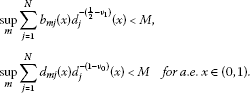
Then, for all $f(x)={\{f_m(x)\}}_1^N\in L^p(0,1;l_q)$, $\lambda \in S(\phi )$ and for sufficiently large $|\lambda |$, the problem (32)-(33) has a unique solution $u={\{u_m(x)\}}_1^{\mathrm{\infty }}$ belonging to $W^{2,p}((0,1),l_q(D),l_q)$ and the following coercive estimate holds:

$$\sum _{i=0}^2{s}^{\frac{i}{2}}|\lambda {|}^{1-\frac{i}{2}}{\parallel \frac{d^{i}u}{d{x}^i}\parallel }_{L^p(0,1;l_q)}+{\parallel Au\parallel }_{L^p(0,1;l_q)}\le C{\parallel f\parallel }_{L^p(0,1;l_q)}.$$

(34)

Proof Really, let $E=l_q$, A and $A_k(x)$ be infinite matrices such that

$$A=[d_m(x){\delta }_{jm}],A_0(x)=[d_{mj}(x)],A_1(x)=[b_{mj}(x)],m,j=1,2,\dots ,\mathrm{\infty }.$$

It is clear that the operator A is R-positive in $l_q$. Therefore, by Theorem 4, the problem (32)-(33) has a unique solution $u\in W^{2,p}((0,1);l_q(D),l_q)$ for all $f\in L^p((0,1);l_q)$, $\lambda \in S(\phi )$ the estimate (34) holds. □

Remark 3 There are many positive operators in different concrete Banach spaces. Therefore, putting concrete Banach spaces and concrete positive operators (i.e., pseudo-differential operators or finite or infinite matrices for instance) instead of E and A, respectively, by virtue of Theorem 4, 5, we can obtain a different class of maximal regular BVPs for partial differential or pseudo-differential equations or their finite and infinite systems with VMO coefficients.

References

Sarason D: On functions of vanishing mean oscillation. Trans. Am. Math. Soc. 1975, 207: 391–405.
Chiarenza F, Frasca M, Longo P: Interior estimates for non divergence elliptic equations with discontinuous coefficients. Ric. Mat. 1991, 40: 149–168.
Chiarenza F, Frasca M, Longo P: -solvability of the Dirichlet problem for nondivergence elliptic equations with VMO coefficients. Trans. Am. Math. Soc. 1993, 336(2):841–853.
Chiarenza F: regularity for systems of PDEs with coefficients in VMO. 5. In Nonlinear Analysis, Function Spaces and Applications. Prometheus, Prague; 1994.
Miranda C: Partial Differential Equations of Elliptic Type. Springer, Berlin; 1970.
Maugeri A, Palagachev DK, Softova L: Elliptic and Parabolic Equations with Discontinuous Coefficients. Wiley, Berlin; 2000.
Krylov NV: Parabolic and elliptic equations with VMO coefficients. Commun. Partial Differ. Equ. 2007, 32(3):453–475. 10.1080/03605300600781626
Amann H 1. In Linear and Quasi-Linear Problems. Birkhäuser, Boston; 1995.
Ashyralyev A: On well-posedeness of the nonlocal boundary value problem for elliptic equations. Numer. Funct. Anal. Optim. 2003, 24(1–2):1–15. 10.1081/NFA-120020240
Denk R, Hieber M, Prüss J: R -boundedness, Fourier multipliers and problems of elliptic and parabolic type. Mem. Am. Math. Soc. 2003., 166: Article ID 788
Favini A, Shakhmurov V, Yakubov Y: Regular boundary value problems for complete second order elliptic differential-operator equations in UMD Banach spaces. Semigroup Forum 2009, 79(1):22–54. 10.1007/s00233-009-9138-0
Gorbachuk VI, Gorbachuk ML: Boundary Value Problems for Differential-Operator Equations. Naukova Dumka, Kiev; 1984.
Heck H, Hieber M: Maximal -regularity for elliptic operators with VMO -coefficients. J. Evol. Equ. 2003, 3: 62–88.
Lions JL, Peetre J: Sur une classe d’espaces d’interpolation. Publ. Math. 1964, 19: 5–68.
Ragusa MA: Necessary and sufficient condition for VMO function. Appl. Math. Comput. 2012, 218(24):11952–11958. 10.1016/j.amc.2012.06.005
Ragusa MA: Embeddings for Morrey-Lorentz spaces. J. Optim. Theory Appl. 2012, 154(2):491–499. 10.1007/s10957-012-0012-y
Sobolevskii PE: Inequalities coerciveness for abstract parabolic equations. Dokl. Akad. Nauk SSSR 1964, 57(1):27–40.
Shakhmurov VB: Coercive boundary value problems for regular degenerate differential-operator equations. J. Math. Anal. Appl. 2004, 292(2):605–620. 10.1016/j.jmaa.2003.12.032
Shakhmurov VB: Separable anisotropic differential operators and applications. J. Math. Anal. Appl. 2007, 327(2):1182–1201. 10.1016/j.jmaa.2006.05.007
Shakhmurov VB: Degenerate differential operators with parameters. Abstr. Appl. Anal. 2007, 2006: 1–27.
Segovia C, Torrea JL: Vector-valued commutators and applications. Indiana Univ. Math. J. 1989, 38(4):959–971. 10.1512/iumj.1989.38.38044
Triebel H: Interpolation Theory. Function Spaces. Differential Operators. North-Holland, Amsterdam; 1978.
Weis L: Operator-valued Fourier multiplier theorems and maximal regularity. Math. Ann. 2001, 319: 735–758. 10.1007/PL00004457
Yakubov S, Yakubov Ya: Differential-Operator Equations. Ordinary and Partial Differential Equations. Chapman & Hall/CRC, Boca Raton; 2000.
John F, Nirenberg L: On functions of bounded mean oscillation. Commun. Pure Appl. Math. 1961, 14: 415–476. 10.1002/cpa.3160140317
Burkholder DL: A geometric condition that implies the existence of certain singular integrals of Banach-space-valued functions. In Conference on harmonic analysis in honor of Antoni Zygmund, Vol. I, II. Wadsworth, Belmont; 1983:270–286. Chicago, Ill., 1981
Hytönen T, Weis L: A T 1 theorem for integral transformations with operator-valued kernel. J. Reine Angew. Math. 2006, 599: 155–200.
Shakhmurov VB: Embedding theorems and maximal regular differential operator equations in Banach-valued function spaces. J. Inequal. Appl. 2005, 4: 605–620.
Blasco O: Operator valued BMO commutators. Publ. Mat. 2009, 53(1):231–244.
Shakhmurov VB, Shahmurova A: Nonlinear abstract boundary value problems atmospheric dispersion of pollutants. Nonlinear Anal., Real World Appl. 2010, 11: 932–951. 10.1016/j.nonrwa.2009.01.037
Grisvard P: Elliptic Problems in Nonsmooth Domains. Pitman, London; 1985.
Besov OV, Ilin VP, Nikolskii SM: Integral Representations of Functions and Embedding Theorems. Nauka, Moscow; 1975.
Author information
Authors and Affiliations
Corresponding author
Additional information
Competing interests
The author declares that he has no competing interests.
Rights and permissions
Open Access This article is distributed under the terms of the Creative Commons Attribution 2.0 International License (https://creativecommons.org/licenses/by/2.0), which permits unrestricted use, distribution, and reproduction in any medium, provided the original work is properly cited.
About this article
Cite this article
Shakhmurov, V.B. Linear and nonlinear abstract elliptic equations with VMO coefficients and applications. Fixed Point Theory Appl 2013, 6 (2013). https://doi.org/10.1186/1687-1812-2013-6
Received:
Accepted:
Published:
DOI: https://doi.org/10.1186/1687-1812-2013-6