On ε-optimality conditions for multiobjective fractional optimization problems

Abstract

A multiobjective fractional optimization problem (MFP), which consists of more than two fractional objective functions with convex numerator functions and convex denominator functions, finitely many convex constraint functions, and a geometric constraint set, is considered. Using parametric approach, we transform the problem (MFP) into the non-fractional multiobjective convex optimization problem (NMCP) _v with parametric v ∈ ℝ ^p , and then give the equivalent relation between (weakly) ε-efficient solution of (MFP) and (weakly) -efficient solution of . Using the equivalent relations, we obtain ε- optimality conditions for (weakly) ε- efficient solution for (MFP). Furthermore, we present examples illustrating the main results of this study.

2000 Mathematics Subject Classification: 90C30, 90C46.

1 Introduction

We need constraint qualifications (for example, the Slater condition) on convex optimization problems to obtain optimality conditions or ε- optimality conditions for the problem.

To get optimality conditions for an efficient solution of a multiobjective optimization problem, we often formulate a corresponding scalar problem. However, it is so difficult that such scalar program satisfies a constraint qualification which we need to derive an optimality condition. Thus, it is very important to investigate an optimality condition for an efficient solution of a multiobjective optimization problem which holds without any constraint qualification.

Jeyakumar et al. [1, 2], Kim et al. [3], and Lee et al. [4], gave optimality conditions for convex (scalar) optimization problems, which hold without any constraint qualification. Very recently, Kim et al. [5] obtained ε- optimality theorems for a convex multiobjective optimization problem. The purpose of this article is to extend the ε- optimality theorems of Kim et al. [5] to a multiobjective fractional optimization problem (MFP).

Recently, many authors [5–15] have paid their attention to investigate properties of (weakly) ε- efficient solutions, ε- optimality conditions, and ε- duality theorems for multiobjective optimization problems, which consist of more than two objective functions and a constrained set.

In this article, an MFP, which consists of more than fractional objective functions with convex numerator functions, and convex denominator functions and finitely many convex constraint functions and a geometric constraint set, is considered. We discuss ε- efficient solutions and weakly ε- efficient solutions for (MFP) and obtain ε- optimality theorems for such solutions of (MFP) under weakened constraint qualifications. Furthermore, we prove ε- optimality theorems for the solutions of (MFP) which hold without any constraint qualifications and are expressed by sequences, and present examples illustrating the main results obtained.

2 Preliminaries

Now, we give some definitions and preliminary results. The definitions can be found in [16–18]. Let g : ℝ ⁿ → ℝ ∪ {+∞} be a convex function. The subdifferential of g at a is given by

where domg: = {x ∈ ℝ ⁿ | g(x) < ∞} and ⟨·, ·⟩ is the scalar product on ℝ ⁿ . Let ε ≧ 0. The ε- subdifferential of g at a ∈ domg is defined by

The conjugate function of g : ℝ ⁿ → ℝ ∪ {+∞} is defined by

The epigraph of g, epig, is defined by

For a nonempty closed convex set C ⊂ ℝ ⁿ , δ _C : ℝ ⁿ → ℝ ∪ {+∞} is called the indicator of C if .

Lemma 2.1[19]If h : ℝ ⁿ → ℝ ∪ {+∞} is a proper lower semicontinuous convex function and if a ∈ domh, then

Lemma 2.2[20]Let h : ℝ ⁿ → ℝ be a continuous convex function and u : ℝ ⁿ → ℝ ∪ {+∞} be a proper lower semicontinuous convex function. Then

Now, we give the following Farkas lemma which was proved in [2, 5], but for the completeness, we prove it as follows:

Lemma 2.3 Let h _i : ℝ ⁿ → ℝ, i = 0, 1, ⋯, l be convex functions. Suppose that {x ∈ ℝ ⁿ | h _i (x) ≦ 0, i = 1, ⋯, l} ≠ ∅. Then the following statements are equivalent:

(i) {x ∈ ℝ ⁿ | h _i (x) ≦ 0, i = 1, ..., l} ⊆ {x ∈ ℝ ⁿ | h₀(x) ≧ 0}

(ii).

Proof. Let Q = {x ∈ ℝ ⁿ | h _i (x) ≦ 0, i = 1, ..., l}. Then Q ≠ ∅ and by Lemma 2.1 in [2], . Hence, by Lemma 2.2, we can verify that (i) if and only if (ii).

Lemma 2.4[16]Let h _i : ℝ ⁿ → ℝ ∪ {+∞}, i =, 1, ⋯, m be proper lower semi-continuous convex functions. Let ε ≧ 0. if, where ri domh _i is the relative interior of domh _i , then for all,

3 ε-optimality theorems

Consider the following MFP:

Let f _i : ℝ ⁿ → ℝ, i = 1, ..., p be convex functions, g _i : ℝ ⁿ → ℝ, i = 1, ..., p, concave functions such that for any x ∈ Q, f _i (x) ≧ 0 and g _i (x) > 0, i = 1, ..., p, and h _j : ℝ ⁿ → ℝ, j = 1, ..., m, convex functions. Let ε = (ε₁, ..., ε _p ), where ε _i ≧ 0, i = 1, ..., p.

Now, we give the definition of ε- efficient solution of (MFP) which can be found in [11].

Definition 3.1 The pointis said to be an ε-efficient solution of (MFP) if there does not exist x ∈ Q such that

When ε = 0, then the ε- efficiency becomes the efficiency for (MFP) (see the definition of efficient solution of a multiobjective optimization problem in [21]).

Now, we give the definition of weakly ε- efficient solution of (MFP) which is weaker than ε- efficient solution of (MFP).

Definition 3.2 A pointis said to be a weakly ε-efficient solution of (MFP) if there does not exist x ∈ Q such that

When ε = 0, then the weak ε- efficiency becomes the weak efficiency for (MFP) (see the definition of efficient solution of a multiobjective optimization problem in [21]).

Using parametric approach, we transform the problem (MFP) into the nonfractional multiobjective convex optimization problem (NMCP) _v with parametric v ∈ ℝ ^p :

Adapting Lemma 4.1 in [22] and modifying Proposition 3.1 in [12], we can obtain the following proposition:

Proposition 3.1 Let. Then the following are equivalent:

(i)is an ε-efficient solution of (MFP).

(ii)is an-efficient solution of , where 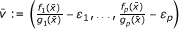and .

(iii) or

where.

Proof. (i) ⇔ (ii): It follows from Lemma 4.1 in [22].

• (ii) ⇒ (iii): Let be an -efficient solution of , where and . Then or . Suppose that . Then for any and all i = 1, . . . p,

  

Hence the -efficiency of yields

for any and all i = 1, ..., p. Thus we have, for all ,

• (iii) ⇒ (ii): Suppose that . Then there does not exist x ∈ Q such that ; that is, there does not exist x ∈ Q such that

  

for all i = 1, ..., p. Hence, there does not exist x ∈ Q such that

Therefore, is an -efficient solution of , where .

Assume that . Then, from this assumption

(3.1)

for any . Suppose to the contrary that is not an -efficient solution of . Then, there exist and an index j such that

Therefore, and , which contradicts the above inequality. Hence, is an -efficient solution of .

We can easily obtain the following proposition:

Proposition 3.2 Letand suppose that. Then the following are equivalent:

(i)is a weakly ε-efficient solution of (MFP).

(ii)is a weakly-efficient solution of, whereand.

(iii) there exists such that

Proof. (i) ⇔ (ii): The proof is also following the similar lines of Proposition 3.1.

• (ii) ⇒ (iii): Let φ(x) = (φ ₁(x), ..., φ _p (x)), ∀x ∈ Q, where . Then, φ _i (x), i = 1,⋯, p, are convex. Since is a weakly ε- efficient solution of , where , 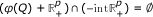, and hence, it follows from separation theorem that there exist , i = 1, ..., p, such that

  

Thus (iii) holds.

• (iii) ⇒ (ii): If (ii) does not hold, that is, is not a weakly -efficient solution of , then (iii) does not hold. □

We present a necessary and sufficient ε-optimality theorem for ε-efficient solution of (MFP) under a constraint qualification, which will be called the closedness assumption.

Theorem 3.1 Letand assume thatandi = 1, ..., p. Suppose that

is closed, where, i = 1, ..., p. Then the following are equivalent.

(i)is an ε-efficient solution of (MFP).

(ii)

(iii) there exist α _i ≧ 0, , β _i ≧ 0, , i = 1, ..., p, λ _j ≧ 0, γ _j ≧ 0, , j = 1, ..., m, μ _i ≧ 0, q _i ≧ 0, , z _i ≧ 0, 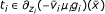i = 1, ..., p such that

and

Proof. Let .

• (i) ⇔ (by Proposition 3.1) h ₀(x) ≧ 0, .

⇔ , i = 1, ..., p, h _j (x) ≦ 0, j = 1, ..., m} ⊂ {x | h₀(x) ≧ 0}.

⇔ (by lemma 2.3)

Thus by the closedness assumption, (i) is equivalent to (ii).

• (ii) ⇔ (iii): (ii) ⇔ (by Lemma 2.1), there exist α _i ≧ 0, , i = 1, ..., p, β _i ≧ 0, , i = 1, ..., p, λ _j ≧ 0, γ _j ≧ 0, , j = 1, ..., m, μ _i ≧ 0, q _i ≧ 0, , i = 1, ..., p, z _i ≧ 0, , i = 1, ..., p such that

  

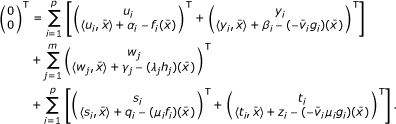
⇔ there exist α _i ≧ 0, , β _i ≧ 0, , i = 1, ..., p, λ _j ≧ 0, γ _j ≧ 0, , j = 1, ..., m, μ _i ≧ 0, q _i ≧ 0, , z _i ≧ 0, i = 1, ..., p such that

and

⇔ (iii) holds. □

Now we give a necessary and sufficient ε-optimality theorem for ε-efficient solution of (MFP) which holds without any constraint qualification.

Theorem 3.2 Let. Suppose thatand, i = 1, ..., p. Thenis an ε-efficient solution of (MFP) if and only if there exist α _i ≧ 0, , i = 1, ..., p, β _i ≧ 0, , i = 1, ..., p, , , , j = 1, ..., m, , , , , , k = 1, ..., p such that

and

Proof. is an ε-efficient solution of (MFP)

⇔ (from the proof of Theorem 3.1)

⇔ (by Lemma 2.1) there exist α _i ≧ 0, , i = 1, ..., p, β _i ≧ 0, , i = 1, ..., p, , , , j = 1, ..., m, , , , , , k = 1, ..., p, such that

⇔ there exist α _i ≧ 0, , i = 1, ..., p, β _i ≧ 0, , i = 1, ..., p, , , , j = 1, ..., m, , , , , , k = 1, ..., p, such that

and

We present a necessary and sufficient ε-optimality theorem for weakly ε-efficient solution of (MFP) under a constraint qualification.

Theorem 3.3 Letand assume that, i = 1, ..., p, andis closed. Then the following are equivalent.

(i)is a weakly ε-efficient solution of (MFP).

(ii) there exist μ _i ≧ 0, i = 1, ..., p, such that

where, i = 1, ..., p.

(iii) there exist μ _i ≧ 0, , α _i ≧ 0, , β _i ≧ 0, , i = 1, ..., p, λ _j ≧ 0, γ _j ≧ 0, , j = 1, ..., m, such that

and

Proof. (i) ⇔ (ii): is a weakly ε-efficient solution of (MFP)

⇔ (by Proposition 3.2) there exist μ _i ≧ 0, i = 1, ..., p, such that

⇔ there exist μ _i ≧ 0, i = 1, ..., p, such that

⇔ (by Lemma 2.3) there exist μ _i ≧ 0, i = 1, ..., p, such that

Thus, by the closedness assumption, (i) is equivalent to (ii).

• (ii) ⇔ (iii): (ii) ⇔ (by Lemma 2.1) there exist μ _i ≧ 0, , α _i ≧ 0, , β _i ≧ 0, , i = 1, ..., p, λ _j ≧ 0, γ _j ≧ 0, , j = 1, ..., m, such that

  

⇔ (iii) holds. □

Now, we propose a necessary and sufficient ε-optimality theorem for weakly ε-efficient solution of (MFP) which holds without any constraint qualification.

Theorem 3.4 Letand assume that. Thenis a weakly ε-efficient solution of (MFP) if and only if there exist μ _i ≧ 0, i = 1, ..., p, , α _i ≧ 0, , i = 1, ..., p, β _i ≧ 0, , i = 1, ..., p, , , , j = 1, ..., m, such that

and

Proof. is a weakly ε-efficient solution of (MFP)

⇔ ((from the proof of Theorem 3.3) there exist μ _i ≧ 0, i = 1, ..., p, such that

⇔ (by Lemma 2.1) there exist μ _i ≧ 0, i = 1, ..., p, , α _i ≧ 0, , i = 1, ..., p, β _i ≧ 0, , i = 1, ..., p, , , , j = 1, ..., m, such that

⇔ there exist μ _i ≧ 0, i = 1, ..., p, , α _i ≧ 0, , i = 1, ..., p, β _i ≧ 0, , i = 1, ..., p, , , , j = 1, ..., m, such that

and

□

Now, we give examples illustrating Theorems 3.1, 3.2, 3.3, and 3.4.

Example 3.1 Consider the following MFP:

Let, and f₁(x₁, x₂) = x₁, g₁(x₁, x₂) = 1, f₂(x₁, x₂) = x₂, g₂(x₁, x₂) = x₁, h₁(x₁, x₂) = -x₁+ 1 and h₂(x₁, x₂) = -x₂ + 1.

(1)Let. Thenis an ε-efficient solution of (MFP)₁.

Letand. Then, and

Thus,. It is clear thatand. Let. Then

where coD is the convexhull of a set D and cone coD is the cone generated by coD. Thus A is closed. Let. Then

B = {(1, 0)} × [0, ∞)+{(0, 0)} × [1, ∞)+{(0, 1)} × [0, ∞)+{(-1, 0)} × [0, ∞)+A. Since (0,-1,-1) ∈ A, (0, 0, 0) ∈ B. Thus (ii) of Theorem 3.1 holds. Let α₁ = β₁ = γ₁ = q₁ = z₁ = α₂ = β₂ = γ₂ = q₂ = z₂ = 0, and let μ₁ = μ₂ = 1, and λ₁ = 0 and λ₁ = 2. Moreover, , , , , , , , , .

Thus,and.

Thus, (iii) of Theorem 3.1 holds.

(2) Let. Thenis not an ε-efficient solution of (MFP)₁, butis a weakly ε-efficient solution of (MFP)₁.

Let. Then

Hence, C is closed. Moreover,, and. Letand. Then,, . Let μ₁ = 1 and μ₂ = 1. Then,

Since (-1, 0,-1) ∈ C, . So, (ii) of Theorem 3.3 holds. Let α₁ = β₁ = γ₁ = α₂ = β₂ = γ₂ = 0, λ₁ = 1 and λ₂ = 0. Then,

and

Thus, (iii) of Theorem 3.3 holds.

Example 3.2 Consider the following MFP:

Let, and f₁(x₁, x₂) = -x₁ + 1, g₁(x₁, x₂) = 1, f₂(x₁, x₂) = x₂, g₂(x₁, x₂) = -x₁ + 1, h₁(x₁, x₂) = [max{0, x₁}]²and h₂(x₁, x₂) = -x₂ + 1.

(1) Let. Then,is an ε-efficient solution of (MFP)₂. Let. Then, clA = cone co{(0, -1, -1), (1, 0, 0), (-1, 0, 0), (1, 1, 1), (0, 0, 1)}. Here, (1, 0, 0) ∈ clA, but (1, 0, 0) ∈ A, where clA is the closure of the set A. Thus, A is not closed. Let Q = {(x₁, x₂) ∈ ℝ ⁿ | h₁(x₁, x₂) ≦ 0, h₂(x₁, x₂) ≦ 0}. Then, . Let, i = 1, 2. Then, . Let α₁ = β₁ = α₂ = β₂ = 0, , , , , . Let u₁ = (-1, 0) u₂ = (0, 1), y₁ = (0, 0) and y₂ = (1, 0). Let, and. Letand. Then, , i = 1, 2, , i = 1, 2, , j = 1, 2, , k = 1, 2, and, k = 1, 2. Moreover,

and

Thus, Theorem 3.2 holds.

(2) Let. Then, is a weakly ε-efficient solution of (MFP)₂, but not an ε-efficient solution of (MFP)₂. Let. Then, clB = cone co{(0, -1, -1), (1, 0, 0), (0, 0, 1)}. However, (1, 0, 0) ∉ B. Thus, B is not closed. Moreover,, . Letand. Then,and. Let μ₁ = 1, μ₂ = 0, α₁ = β₁ = α₂ = β₂ = 0 and . Let, , , , n ∈ ℕ. Then,, , , , . Let u₁ = (-1, 0) and u₂ = y₁ = y₂ = (0, 0). Then,, , , . Letand. Then,and. Thus, , and. Hence, Theorem 3.4 holds.

References

Jeyakumar V, Lee GM, Dinh N: New sequential Lagrange multiplier conditions characterizing optimality without constraint qualification for convex programs. SIAM J Optim 2003,14(2):534–547.
Jeyakumar V, Wu ZY, Lee GM, Dinh N: Liberating the subgradient optimality conditions from constraint qualification. J Global Optim 2006,36(1):127–137.
Kim GS, Lee GM: On ε -approximate solutions for convex semidefinite optimization problems. Taiwanese J Math 2007,11(3):765–784.
Lee GM, Lee JH: ε -Duality theorems for convex semidefinite optimization problems with conic constraints. J Inequal 2010, 13. Art. ID363012
Kim GS, Lee GM: On ε -optimality theorems for convex vector optimization problems. To appear in Journal of Nonlinear and Convex Analysis
Govil MG, Mehra A: ε -Optimality for multiobjective programming on a Banach space. Eur J Oper Res 2004,157(1):106–112.
Gutiárrez C, Jimá B, Novo V: Multiplier rules and saddle-point theorems for Helbig's approximate solutions in convex Pareto problems. J Global Optim 2005,32(3):367–383.
Hamel A: An ε -Lagrange multiplier rule for a mathematical programming problem on Banach spaces. Optimization 2001,49(1–2):137–149.
Liu JC: ε -Duality theorem of nondifferentiable nonconvex multiobjective programming. J Optim Theory Appl 1991,69(1):153–167.
Liu JC: ε -Pareto optimality for nondifferentiable multiobjective programming via penalty function. J Math Anal Appl 1996,198(1):248–261.
Loridan P: Necessary conditions for ε -optimality. Optimality and stability in mathematical programming. Math Program Stud 1982, 19: 140–152.
Loridan P: ε -Solutions in vector minimization problems. J Optim Theory Appl 1984,43(2):265–276.
Strodiot JJ, Nguyen VH, Heukemes N: ε -Optimal solutions in nondifferentiable convex programming and some related questions. Math Program 1983,25(3):307–328.
Yokoyama K: Epsilon approximate solutions for multiobjective programming problems. J Math Anal Appl 1996,203(1):142–149.
Yokoyama K, Shiraishi S: ε -Necessary conditions for convex multiobjective programming problems without Slater's constraint qualification. , in press.
Hiriart-Urruty JB, Lemarechal C: Convex Analysis and Minimization Algorithms, vols. I and II. Springer-Verlag, Berlin; 1993.
Rockafellar RT: Convex Analysis. Princeton University Press, Princeton, NJ; 1970.
Zalinescu C: Convex Analysis in General Vector Space. World Scientific Publishing Co. Pte. Ltd, Singapore; 2002.
Jeyakumar V: Asymptotic dual conditions characterizing optimality for convex programs. J Optim Theory Appl 1997,93(1):153–165.
Jeyakumar V, Lee GM, Dinh N: Characterizations of solution sets of convex vector minimization problems. Eur. J Oper Res 2006,174(3):1380–1395.
Sawaragi Y, Nakayama H, Tanino T: Theory of Multiobjective Optimization. Academic Press, New York; 1985.
Gupta P, Shiraishi S, Yokoyama K: ε -Optimality without constraint qualification for multiobjective fractional problem. J Nonlinear Convex Anal 2005,6(2):347–357.
Acknowledgements
This study was supported by the Korea Science and Engineering Foundation (KOSEF) NRL program grant funded by the Korea government(MEST)(No. ROA-2008-000-20010-0).
Author information
Authors and Affiliations
Corresponding author
Additional information
4 Competing interests
The authors declare that they have no competing interests.
5 Authors' contributions
The authors, together discussed and solved the problems in the manuscript. All Authors read and approved the final manuscript.
Rights and permissions
Open Access This article is distributed under the terms of the Creative Commons Attribution 2.0 International License ( https://creativecommons.org/licenses/by/2.0 ), which permits unrestricted use, distribution, and reproduction in any medium, provided the original work is properly cited.
About this article
Cite this article
Kim, M.H., Kim, G.S. & Lee, G.M. On ε-optimality conditions for multiobjective fractional optimization problems. Fixed Point Theory Appl 2011, 6 (2011). https://doi.org/10.1186/1687-1812-2011-6
Received:
Accepted:
Published:
DOI: https://doi.org/10.1186/1687-1812-2011-6